Image Warping and Mosaicing
CS180 Project 4
A: Taking Pictures
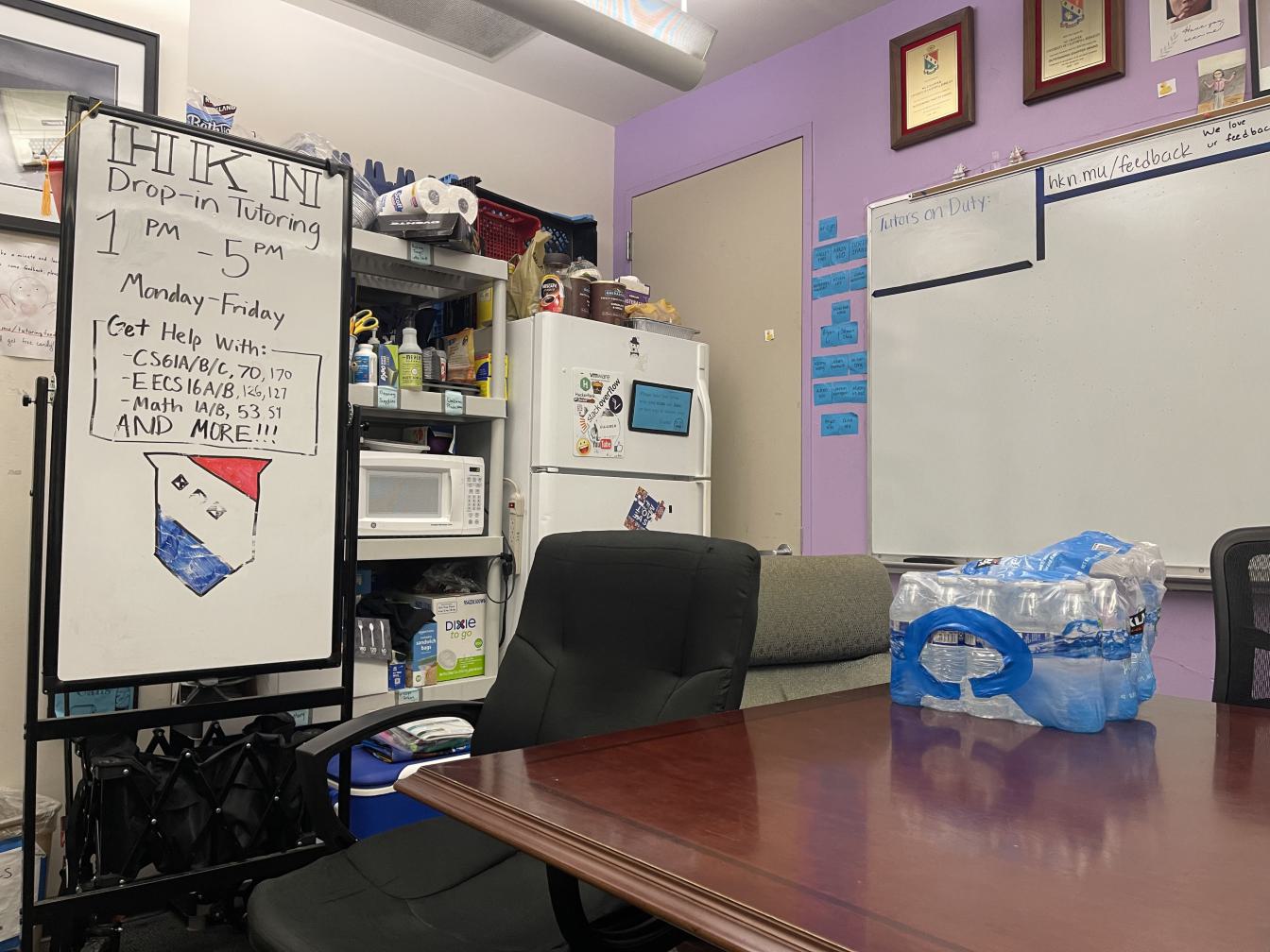
The first part of this project is to take some pictures such that the transform between them is projective. Ideally, I should have used a tripod. However, I did not have access to one, so I did my best to fix the position of my phone camera by pinching my phone with one hand and rotating the phone with the other hand while snapping pictures. Some examples are below.
A: Recover Homographies
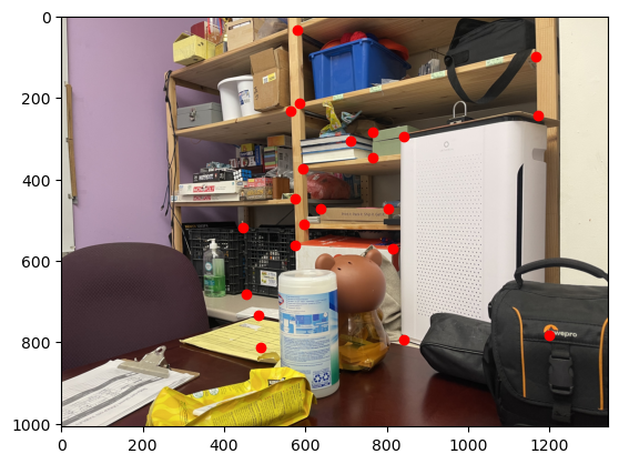
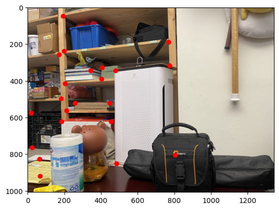
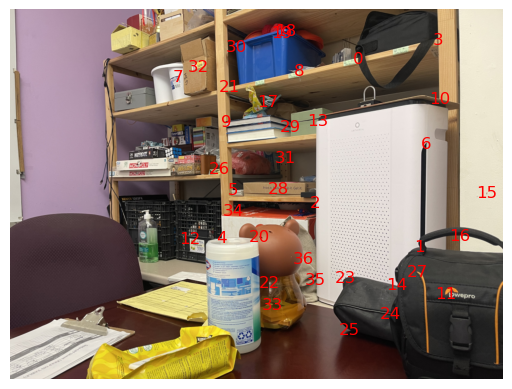
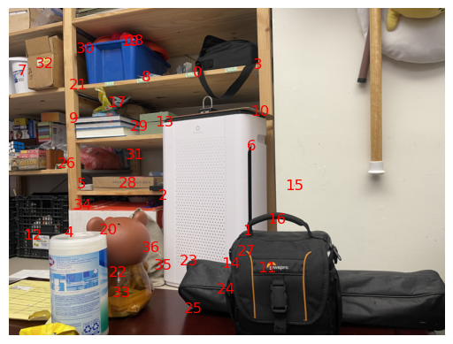
In order to recover the homogrophy between images, I first manually labelled correspondence points between the images using the same tool as project 3. Because these correspondence must be precise, I tried to only label corners to get the exact matching point in both images. Here is an example of the labeled correspondence points:
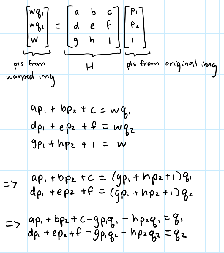
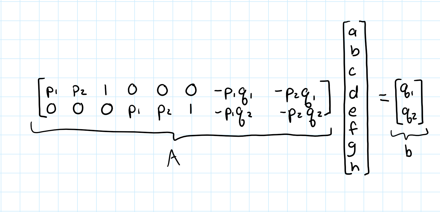
Then, using these corresponding images, we can recover H that transforms a point from the original image, (p1, p2), to a sacled warped point, w * (q1, q2):
A: Warp the Images
After recovering H, I can now warp the images. I matmul H^-1 with all indices of the new image I want to create (the canvas that the final panoramic image will show up on). This will allow me to recover all the indices from the image I want to warp, which I can then use to interpolate the colors from the image using the same function as project 3.
Image Rectification
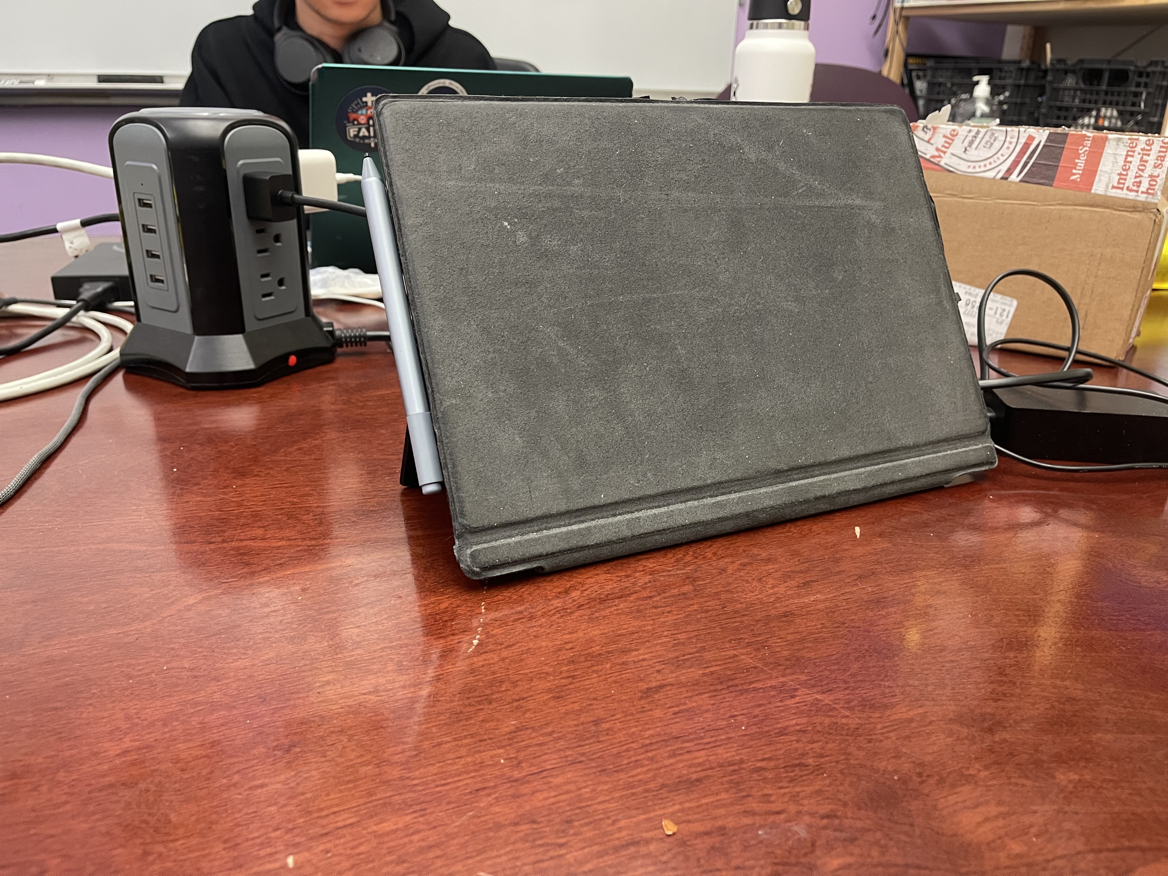
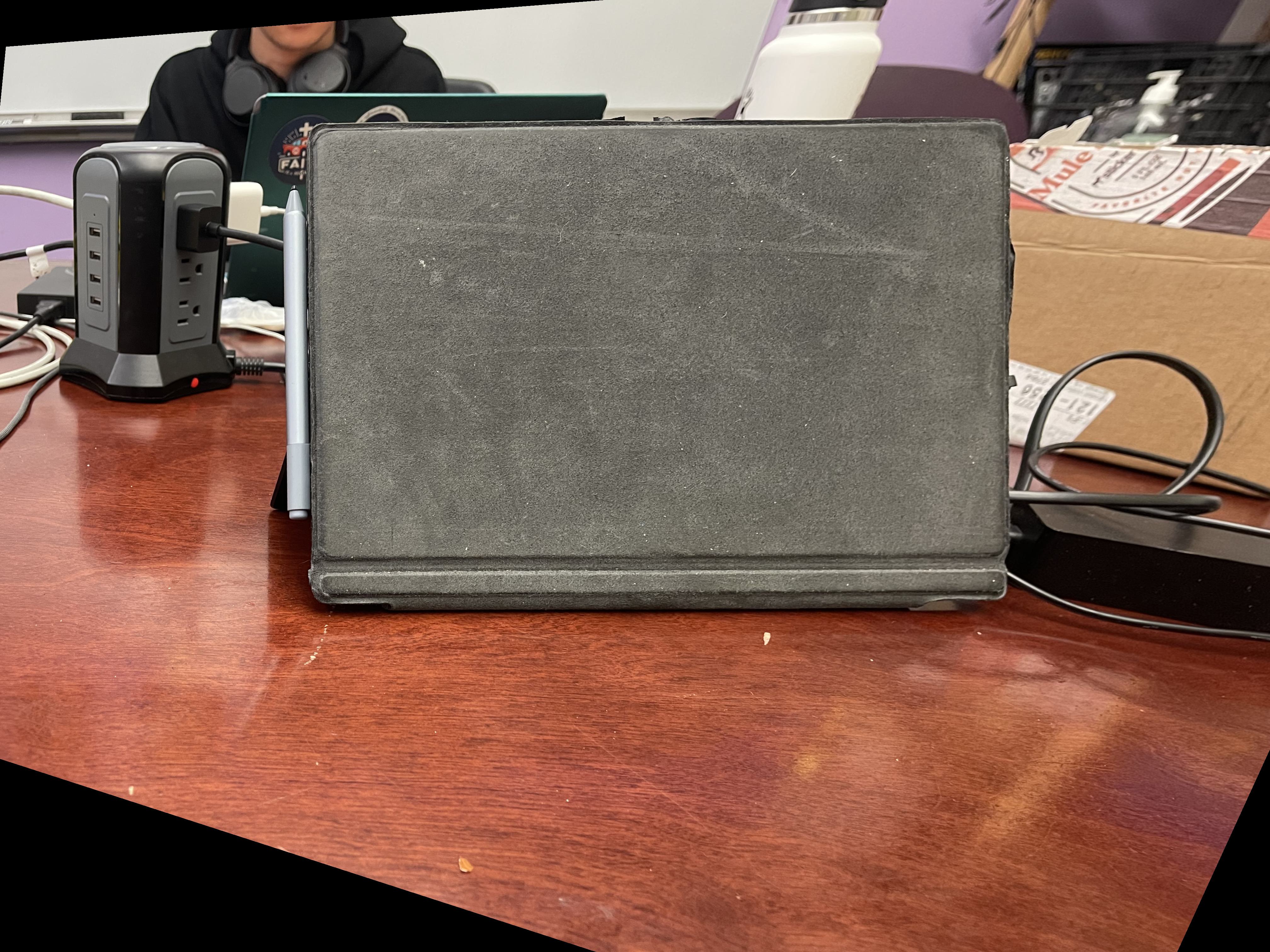
I first perform a sanity check of whether the warp function works by warping an image of rectangular object that was taken from the side into a rectangular shape. Essentially, I am changing the "perspective" of the image to be looking at it from straight on rather than sideways. I do this by finding H using the correspondence points that map the four corners of the object in the image to four chosen points that form a rectangle, and then using the H to warp the image.
A: Blending Images into a Mosaic
Finally, I can stitch images into a mosaic. I do this by choosing one of the images, i, to warp the other image into the orientation of. I create a new image that is N * the shape of i, where N is the number of images that form the mosaic. This way the mosaic has a good amount of every image. Though some of side images are cut off at the ends, when I tried making the mosaic larger, the ends were unproportionally huge and the code took a long time to run, so I just stuck with new_height, new_width = N * imgs[i].shape.
I warp image i onto the center of the new image by first calculating the offset of its correspondence points, correspondence_offset = [(new_width - img_width)//2, (new_height - img_height)//2]. I find the correspondence points of img i on the new image, correspondences_middle_img, by adding correspondence_offset to the original correspondence points of img i. After warping img i to the new img, I can then warp the other images into the center image's orientation and onto a new image with the size N * imgs[i].shape by mapping those img's correspondence points to correspondences_middle_img.
In order to stitch these warped images together, I try two different approaches.
Approach 1: For the first approach I tried, I take all of these warped "new imgs" and then average them together to get the final mosaic. To make the mosaic more seamless, I normalize the colors of the final image. Without normalizing, the parts of the image with the most overlap are the brightest and the parts of the image with the least overlap are the dimmest. Thus, I create a mask such that every pixel has a value j, which is the number of images that overlap. For example, j = 1 if there is one image coloring that pixel, j = 2 if there are two images overlapped for that pixel, etc. I then multiply the final img by N/mask (where mask is nonzero) in order to brighten each pixel of the image inversely with how many overlaps there are.
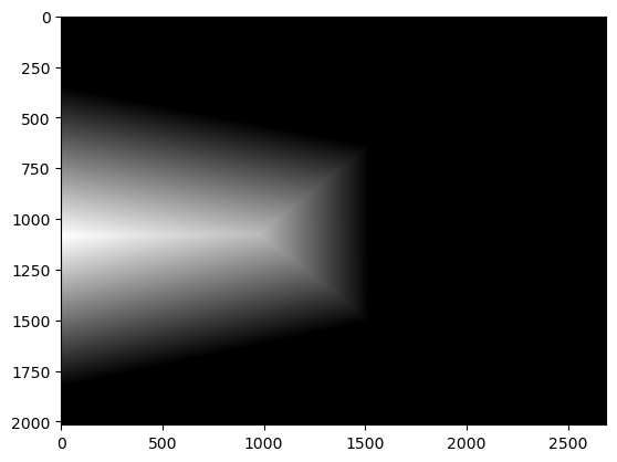
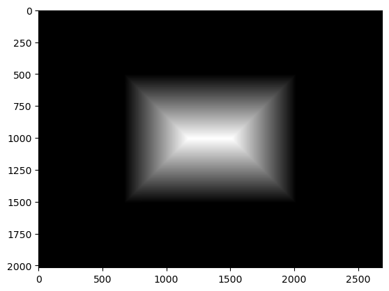
Approach 2: For the second approach I tried, I take the warped imgs and create a binary polygon mask for each of the imgs, where
the image is 1 and the background is 0. I then use cv2.distanceTransform to create a distance transform mask for each of the polygons.
The closer each polygon pixel is to 0 (the background), the closer the distance transform mask pixel is to 0. The mask for blending two warped imgs together
is just distance_transform_mask1 > distance_transform_mask2: 1 where img1's pixel is further from the edge of the img and 0 where img2's pixel is further from the edge.
I then used this mask and the project 2 laplacian stack blending code to blend the images.
Overall, approach 2 gives the imgs a less harsh seem, so that is the approach I went with (even though approach 2 makes the mosaic seem "greyer" than the mosaic stitched using approach 1).
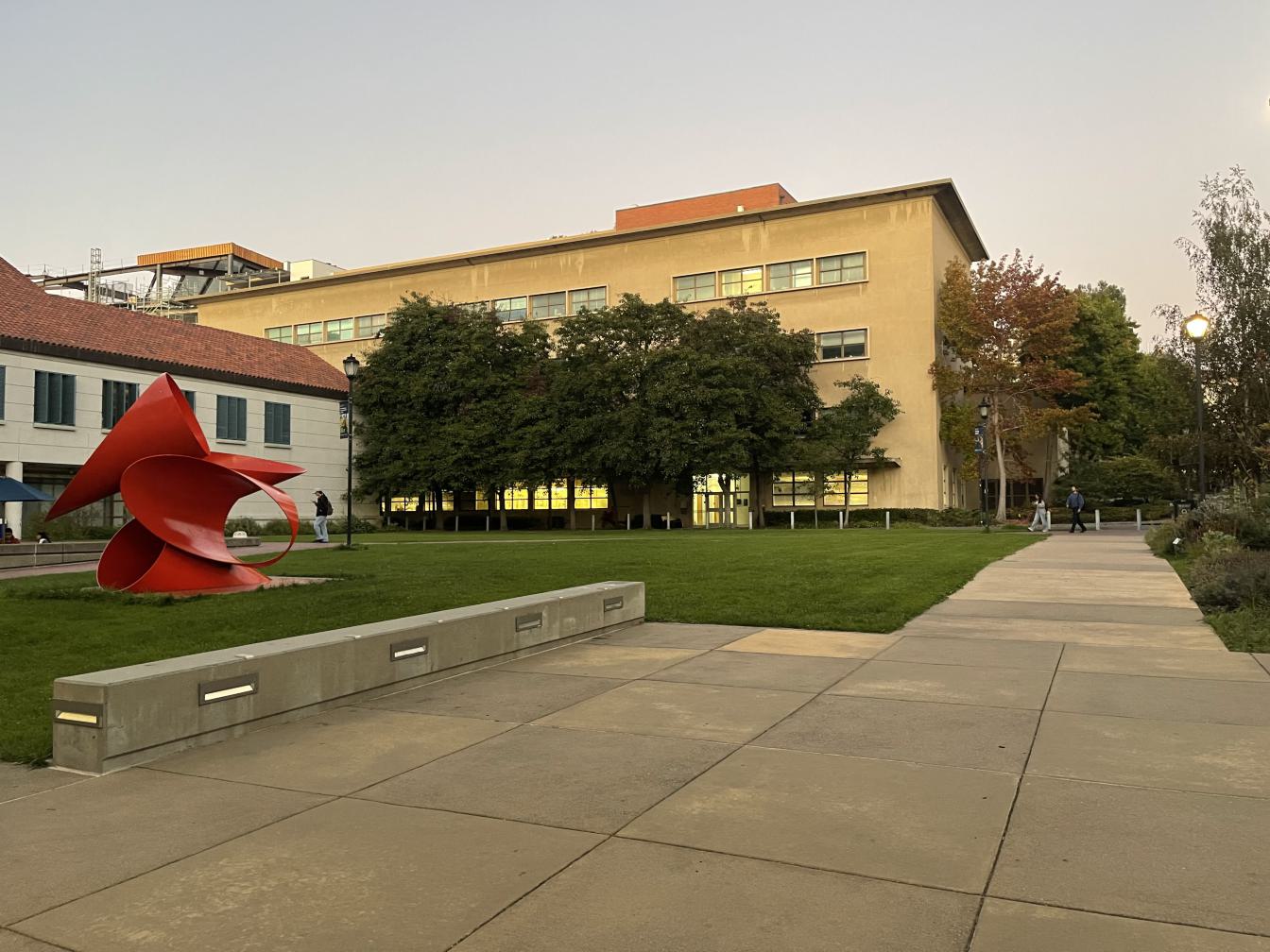
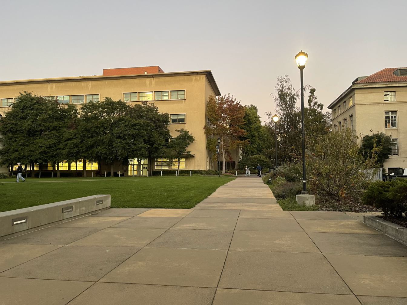
Left image of lawn right outside Li Ka Shing
Right image of lawn right outside Li Ka Shing
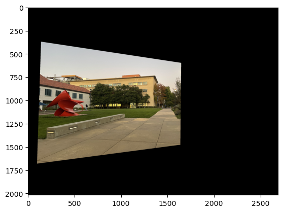
Warped right image
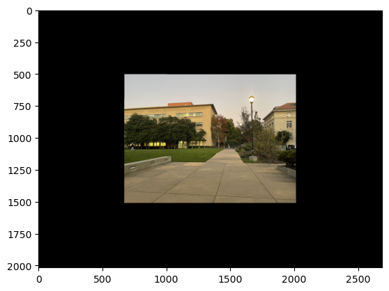
Warped left image
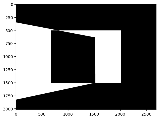
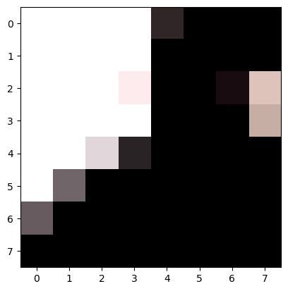
Approach 1 Mask for Normalizing Color

Approach 1 Mosaic
Note some blurriness likely due to imprecisely choosing correspondence points.
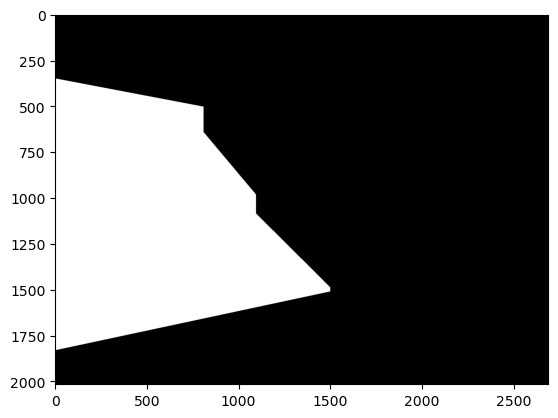
Approach 2 Mask for Blending
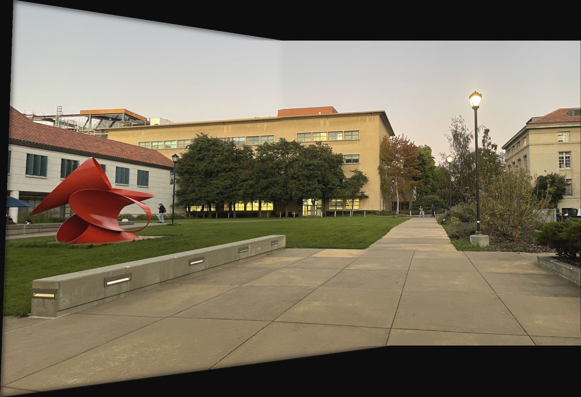
Approach 2 Mosaic
The blurrines of the trees went away, maybe due to blending one of imprecisely warped trees away.
More mosaiced imgs:
Part B
For the image mosaics created by manually selecting correspondence points, some were slightly blurry or a little mismatched at the seam. This is likely due to imprecisely selecting correspondence points, as being just a little off can impact the transform greatly. This issue can be solved by coding an algorithms that can automatically choose and match the correspondence points. This will also save lots of clicking time!
Note: I had to scale down my images for part B since jupyter notebook gave me warnings about not being allowed to allocate enough memory when I had to find pairwise distances for points. This made the functions run very fast but the images are also blurrier than they were in part A.
B: Detecting Corner Features
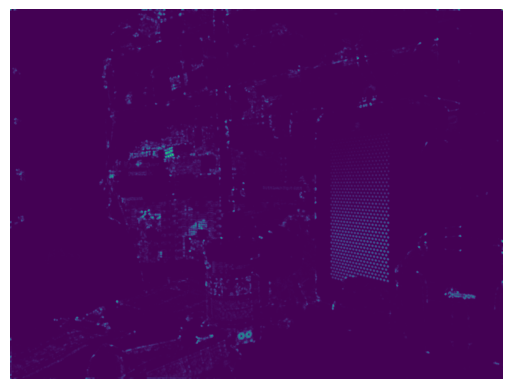
The first step for automatically choosing correspondence points is to use the Harris corner detection algorithm, which calculates the Harris corner response for each pixel, h. The corner points in the img are where the local maxes of these h values are.
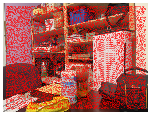
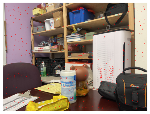
There are way too many points for us to consider, so I filter out most of these points using the Adaptive Non-Maximal Suppression (ANMS) algorithm. This algorithm identifies the strongest corners in the image while keeping the points spread out relatively evenly across the image.
To implement this filtering, I first calculate the pairwise distance for each h point and then create a mask such that each element (i, j) in the mask is set to True only if h_value[i] < c_robust * h_value[j]. I apply this mask to the pairwise distance matrix and set all the zeroed-out distances to infinity. Then I find the minimum radius for each point (minimum distance in each row in the masked pairwise distance matrix) and sort the points from largest to smallest min-radius. The first num_corners points are returned.
B: Extracting a Feature Descriptor
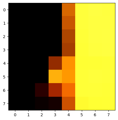
For each corner point in the img, I will extract a feature descriptor in order to match corresponding points between each image. To get the feature descriptors, I first gaussian blur the image to avoid aliasing, slice a 40x40 patch of pixels around the point, and resize the patch to be 8x8. I flatten the feature and then normalize it by subtracting each feature from its mean and dividing by its standard deviation.
Here are some examples of features from the photo above before flattening and normalization:
B: Matching Feature Descriptors
With feature descriptors from two images, I can match up their respective points to get correspondence points between images.
First, I find the pairwise distances matrix, ssd, between the features of img1 and the features of img2: ssd[i,j] is the sum of squares distance between feature1_i and feature2_j. Features of img1 will be denoted as feature1 and features of img2 will be denoted as feature2.
I then use np.argsort on ssd to find the nearest neighbor feature2 for every feature1. However, many of these nearest neighbor pairs are likely not matching points, since there are many points from img 1 that don't have a matching point in img 2. Most of these false matches can be filtered out using lowe's ratio test. For every feature in feature1, I calculate the lowe_value: the distance to its first nearest neighbor / the distance to its second nearest neibor. I filter out all feature pairs whose lowe_value >= lowe_threshold. The idea is that for a real match, the first nearest neighbor will be much closer than the second nearest neighbor, so its lowe value will be very small.
Finally, I take the remaining feature pairs and return their respective corner points. These corner points are the correspondence points between the images!
Examples of some correspondence points after being filtered with a lowe_threshold of .7:
Examples of some matching features between the office imgs:
B: Robust Homographies (RANSAC)
Though most of these correspondence points look pretty good, there are also still some outliers. We cannot directly compute the homography using these points because even a few incorrect points can drastically mess up the warping. Therefore, the RANSAC algorithm must be used to choose only the correct matches.
First, I randomly select 4 correspondence points without replacement. Then, I compute the the homography H using the function from part A. Using this H, img1's points are warped into img2's orientation and unscaled. If correctly warped, these img1 points should be very close to its matching point in img2. So I compute the ssd of the warped img1 pts to its matching img2 point. Any points with an ssd below a ransac_threshold are considered to be "correctly matched". I keep track of these "correctly matched" points and how many of them there are.
After repeating the procedure above for num_samples number of times, I return the set of the largest of correctly matched points. Thus, points that do not follow the majority transformation are discarded and we get the final set of matching correspondence points!
Here is an example of the correspondence points after RANSAC. I only included 1/3 of the points to avoid overcrowding the image, but it can be seen that the outliers from the previous image are no longer present (such as the point matching the hand santizer head to the tape roller).
I used num_samples=1500 and ransac_threshold=2
B: Creating Mosaics
After getting the correspondence points between the images we want to stitch, I can finally stitch images together! I used the same method as part A to compute the homography, warp the images, and blend them together. Here are the images from part A warped using the auto-chosen correspondence points. The blurriness and slight mismatched edges that were present in some of the mosaics from part A are no longer present.
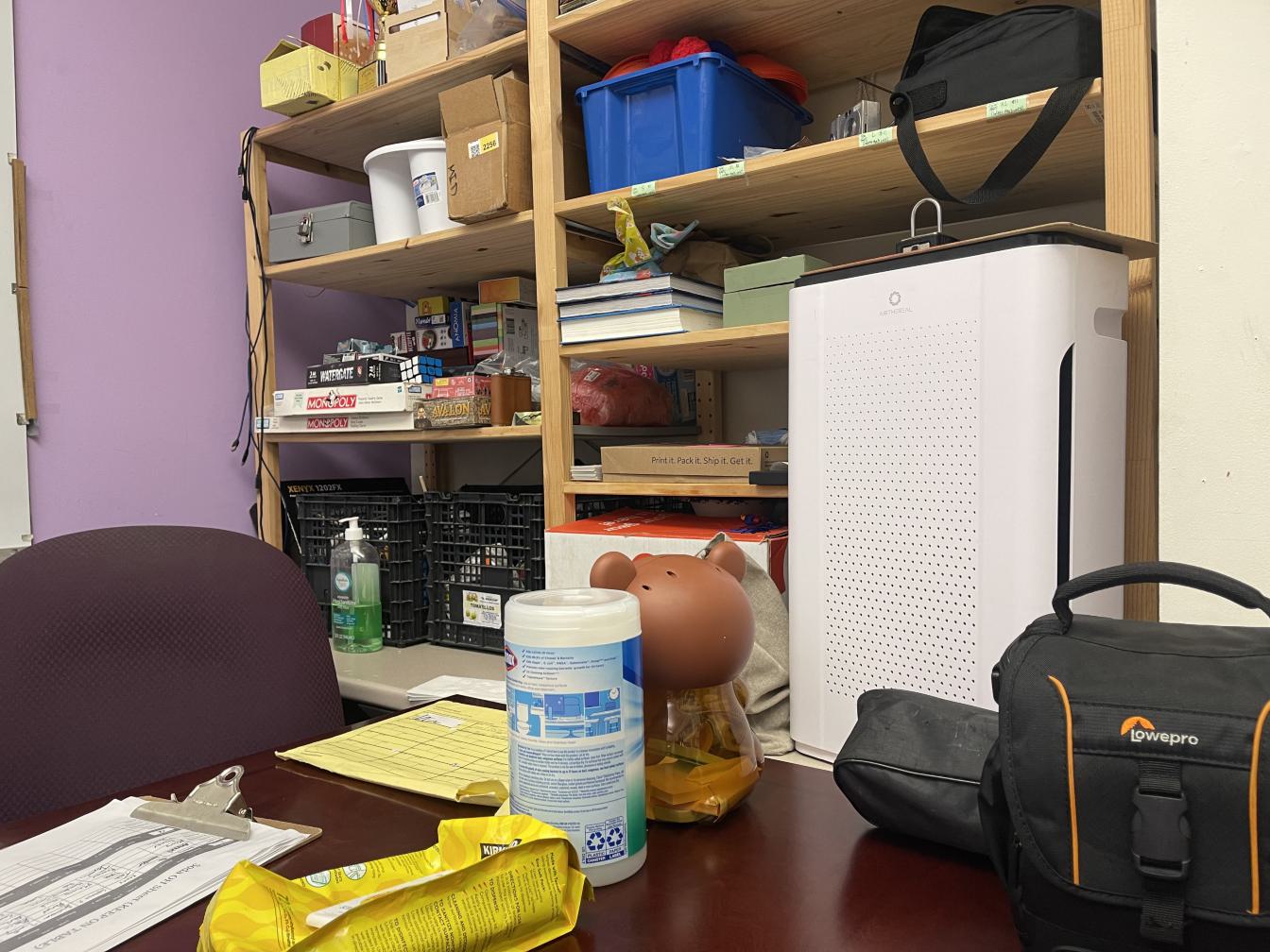
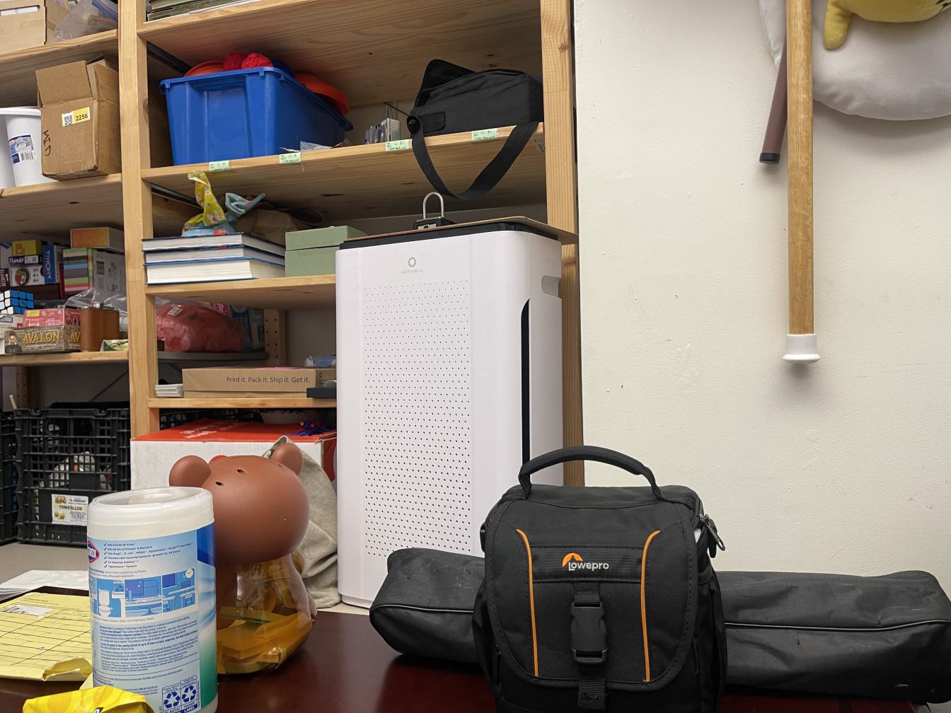
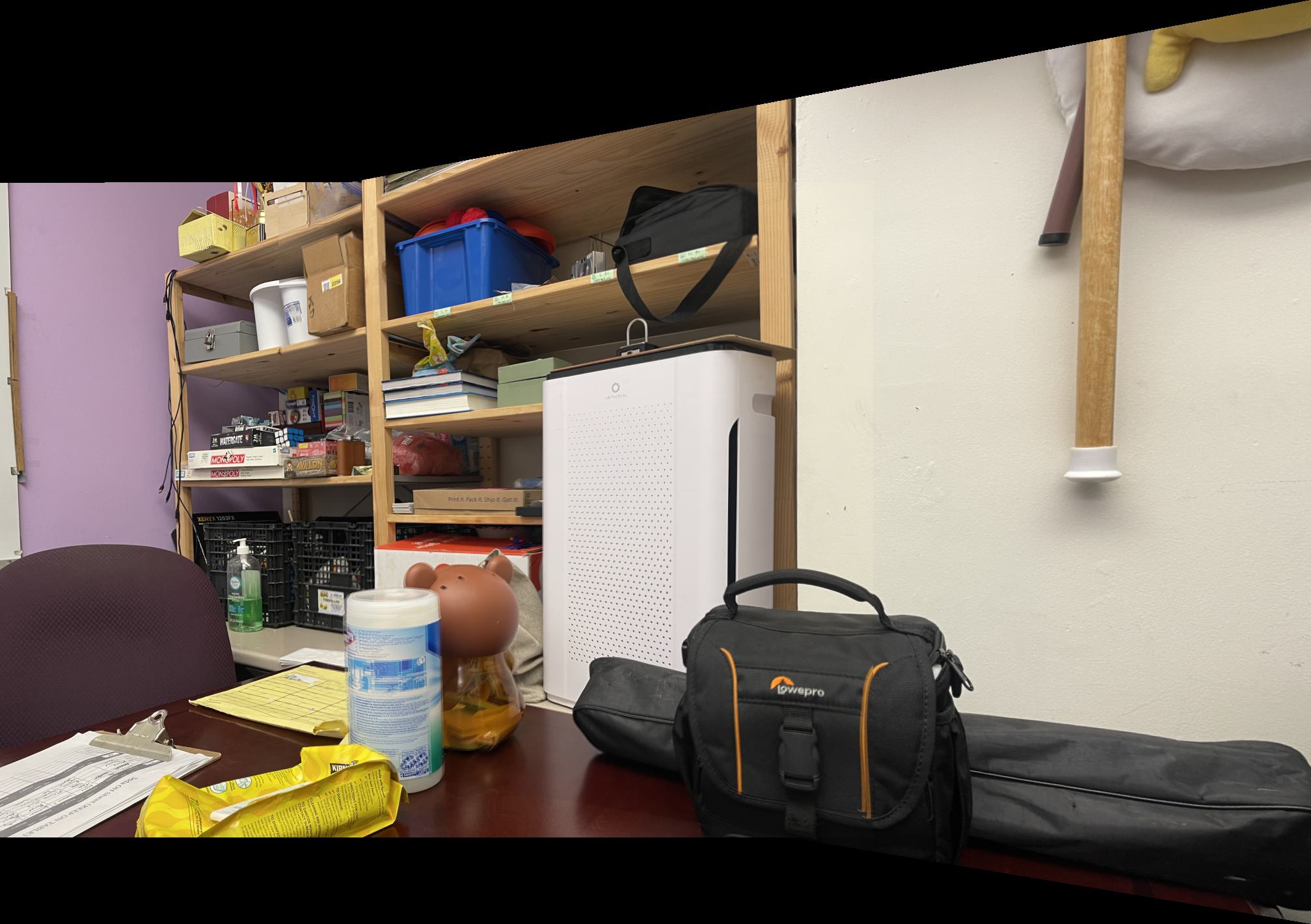
Manually Stitched Mosaic of the HKN Office
The Clorox container is a bit fuzzy.
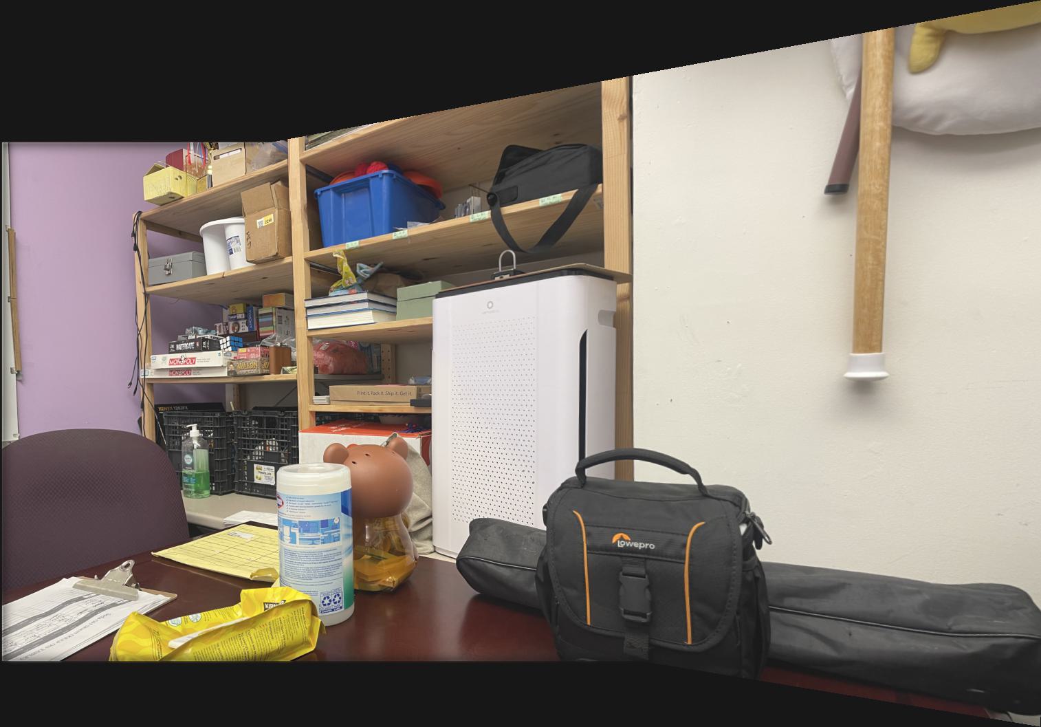
Automatically Stitched Mosaic of the HKN Office
The fuzziness of the Clorox container is no longer present!


Manually Stitched Mosaic of the Lawn Outside Li Ka Shing
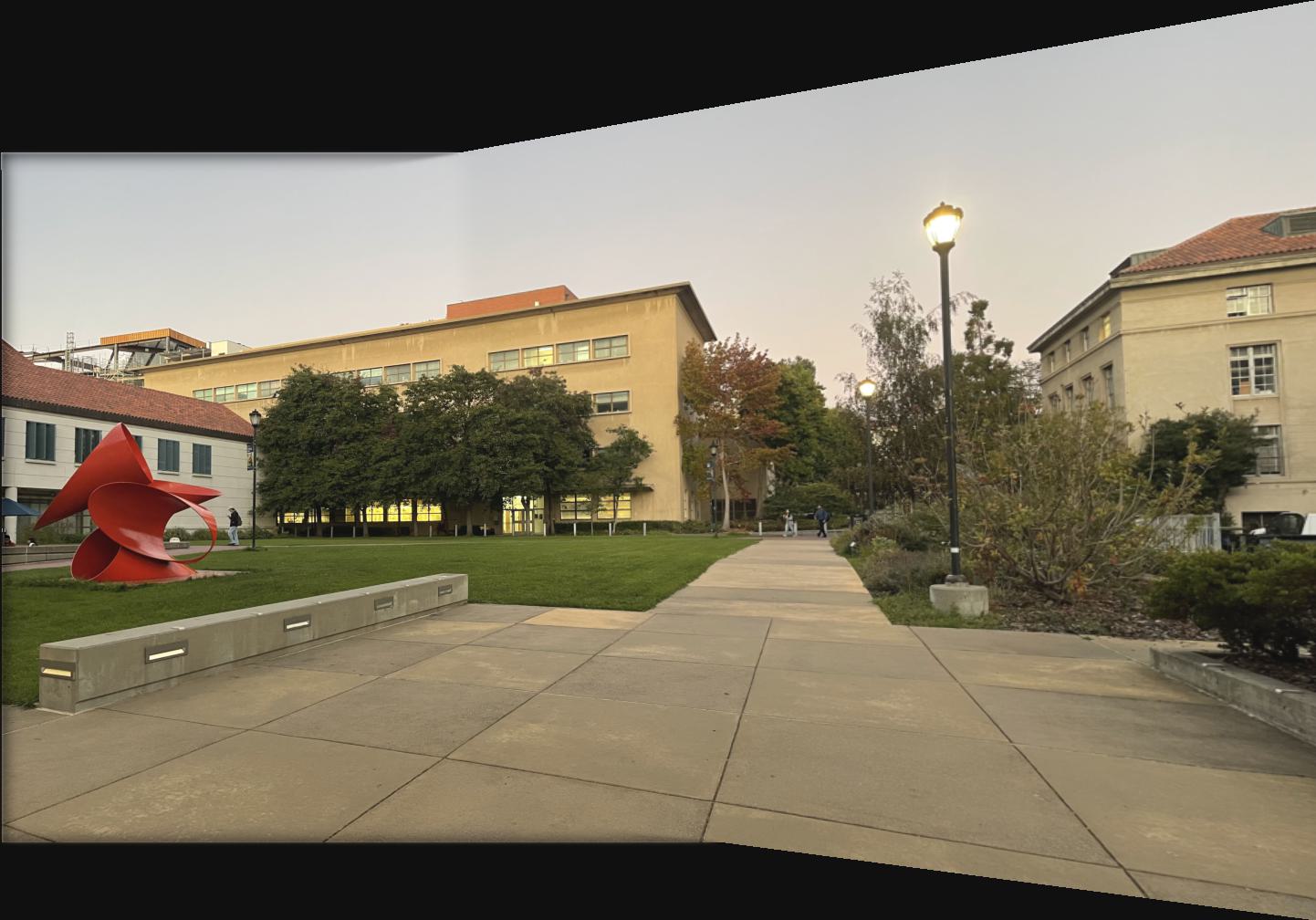
Automatically Stitched Mosaic of the Lawn Outside Li Ka Shing
For this image, I don't see a significant difference.
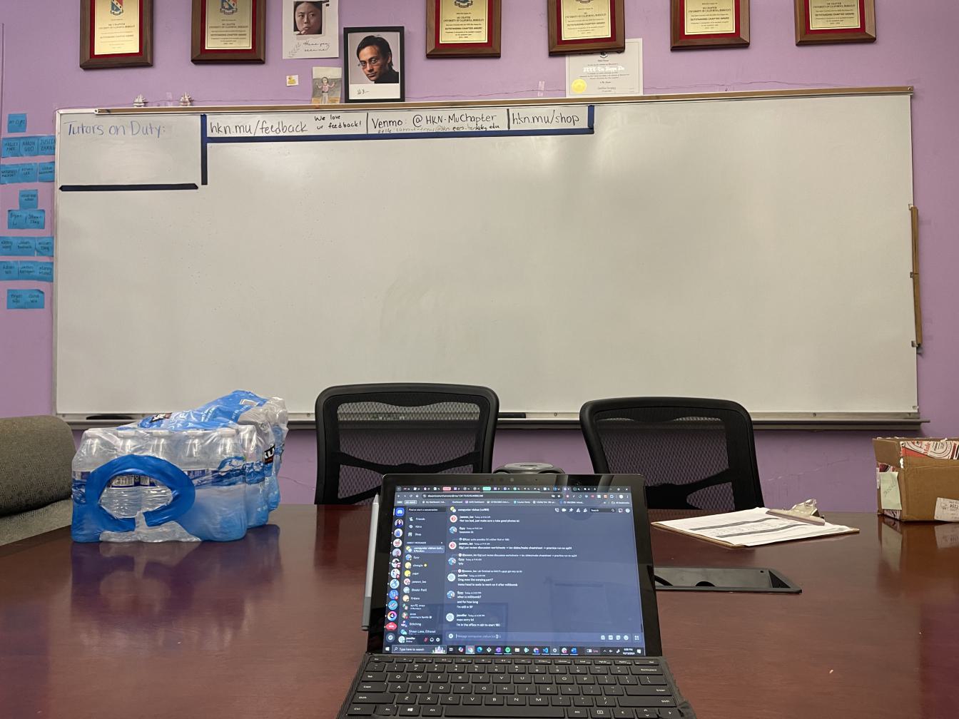

Manually Stitched Mosaic of a Whiteboard
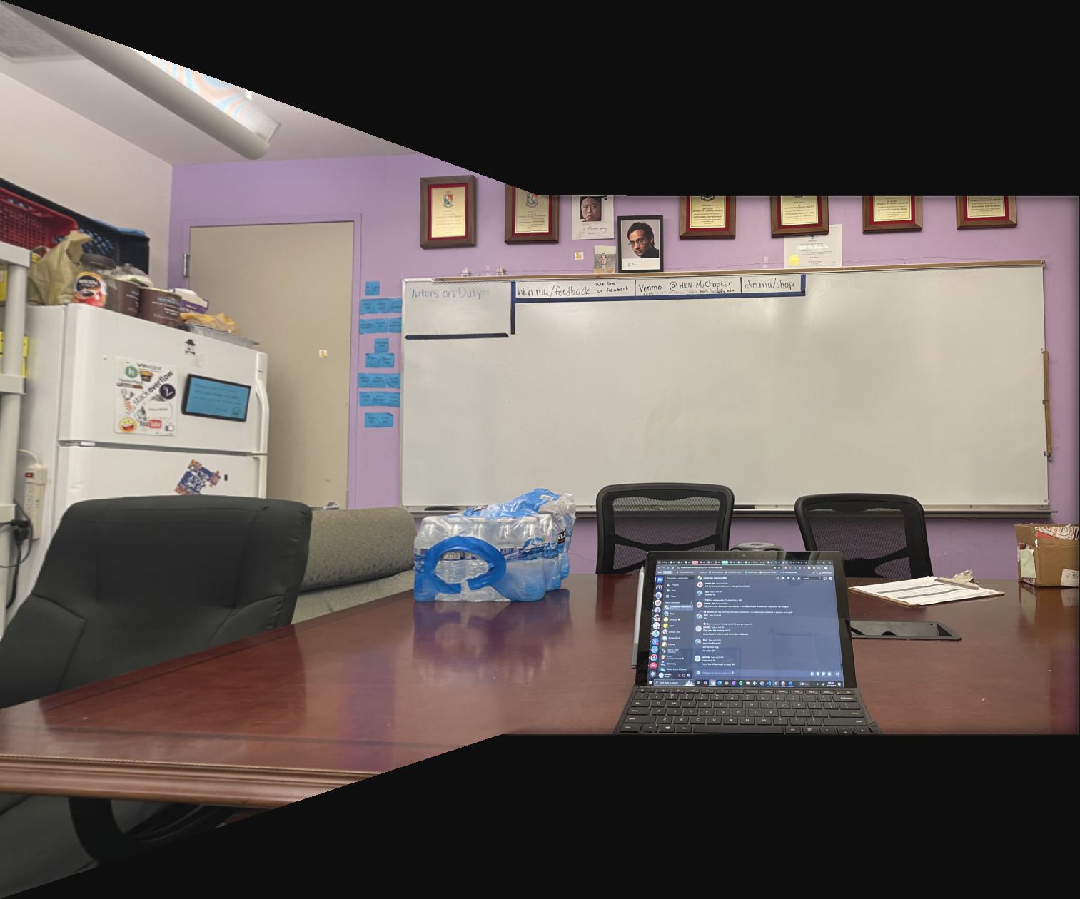
Automatically Stitched Mosaic of a Whiteboard
For this image, I don't see a significant difference.
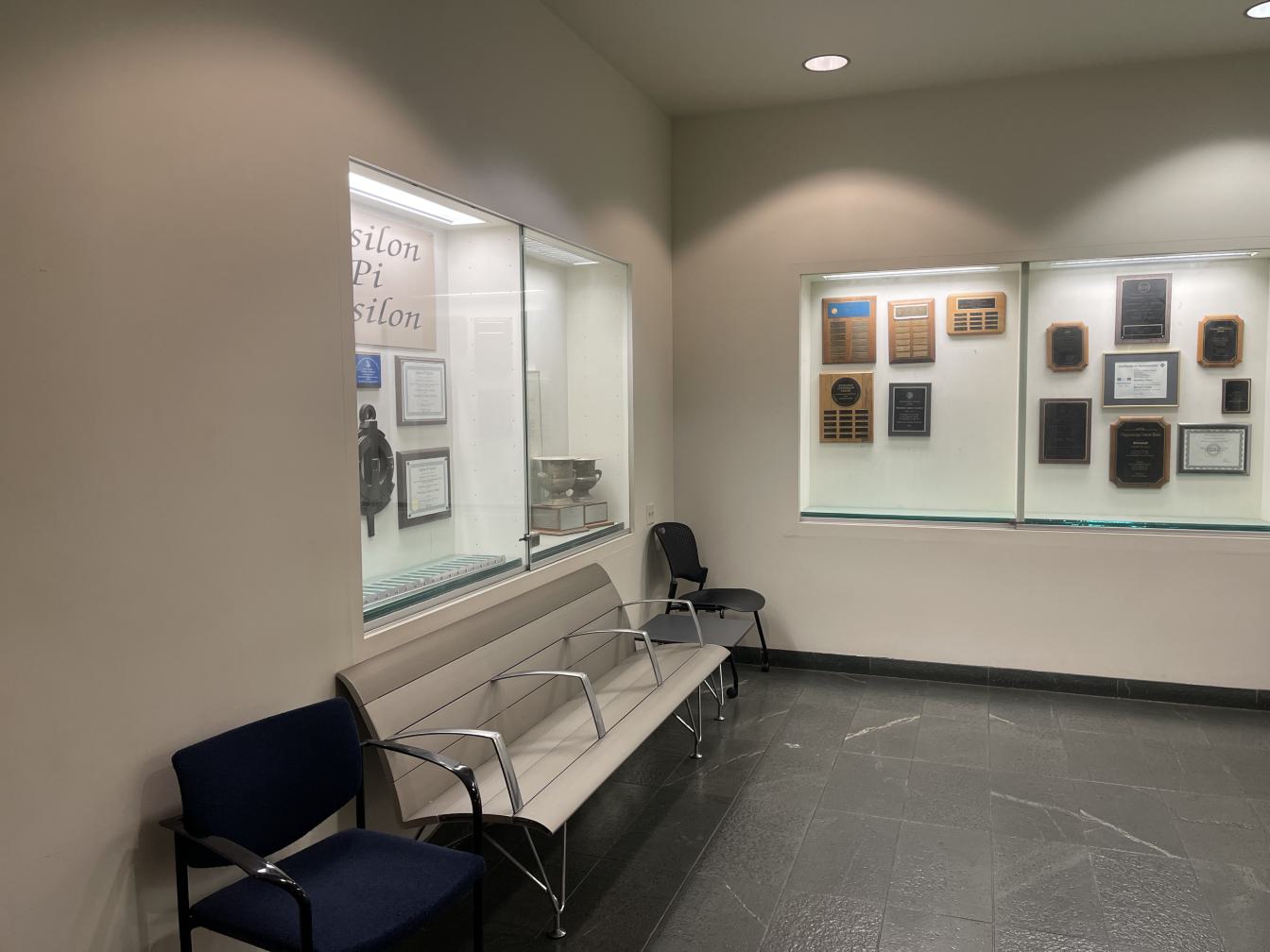
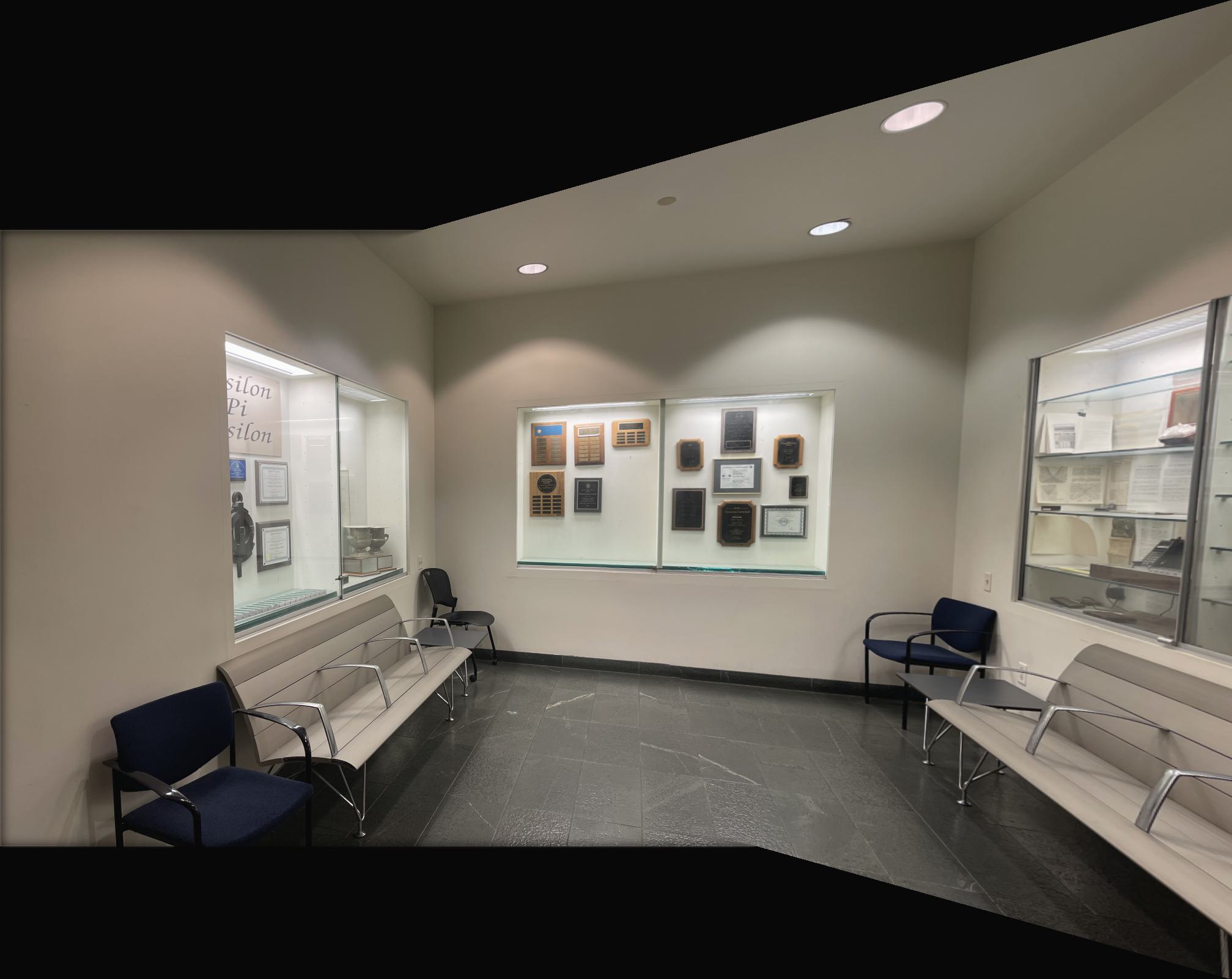
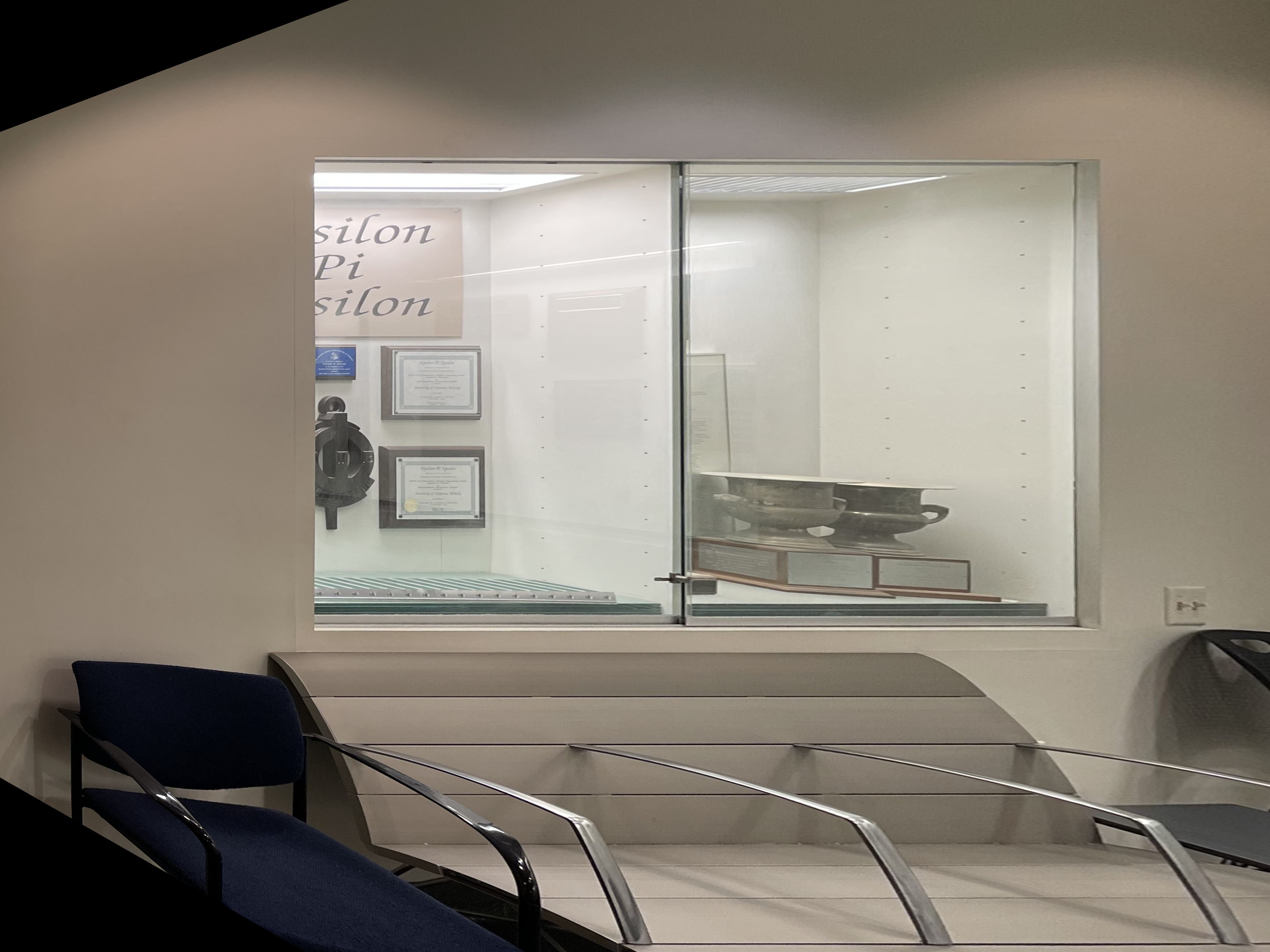
Manually Stitched Mosaic of the Soda Hall Display Case
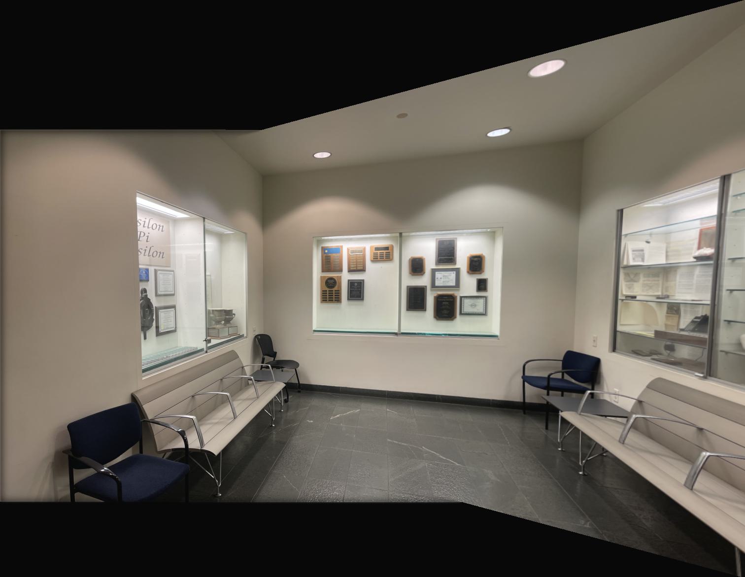
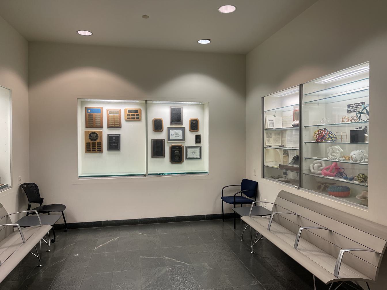
Automatically Stitched Mosaic of the Soda Hall Display Case
For this image, I don't see a significant difference.
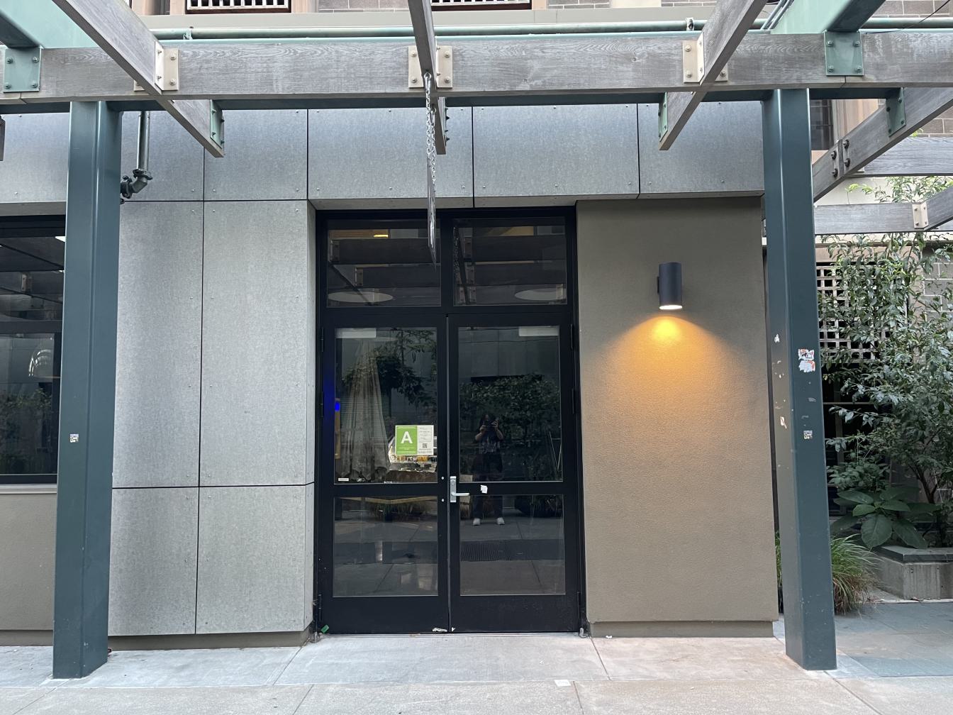
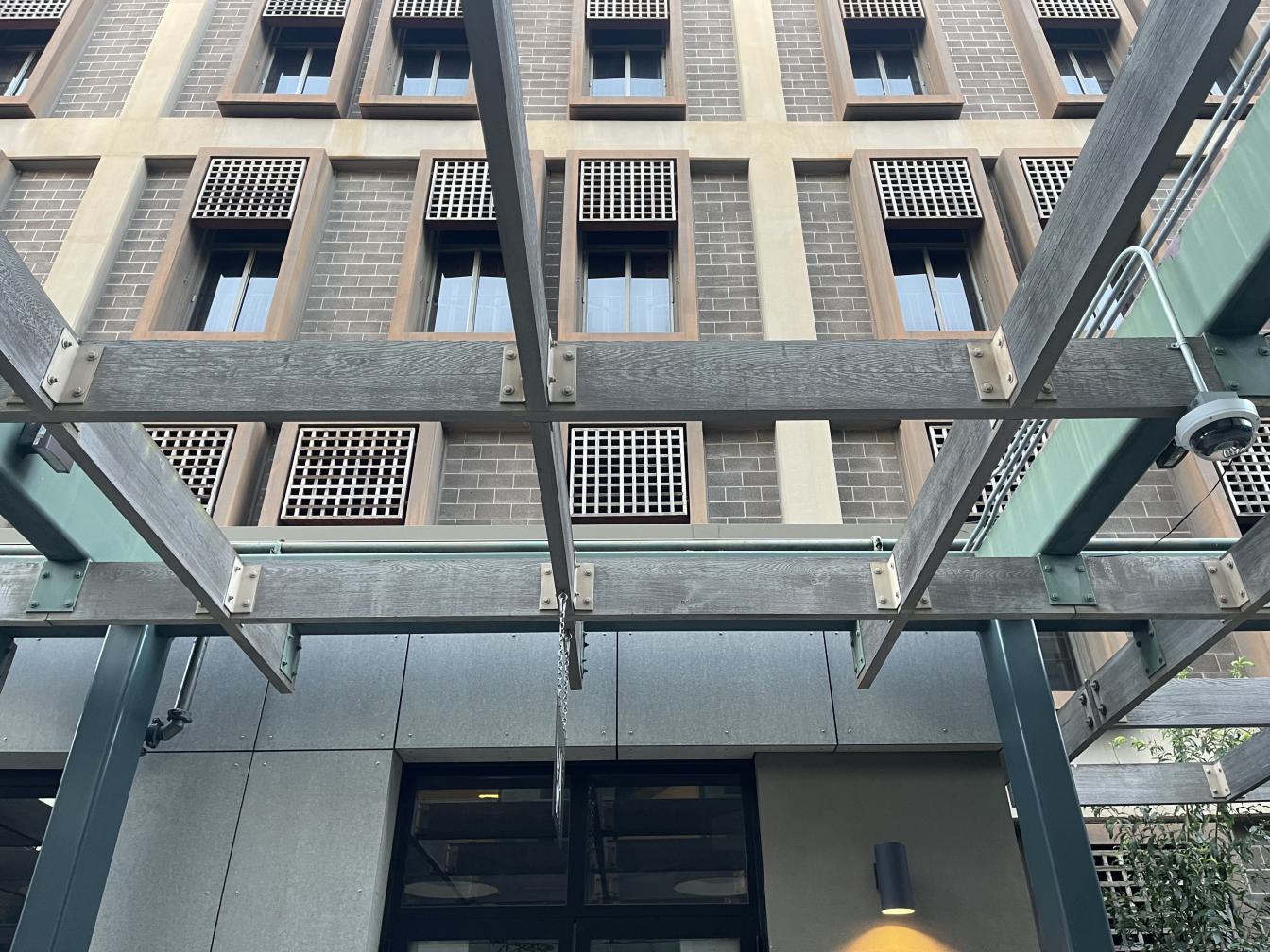

Manually Stitched Mosaic of VA Cafe
There is a slight misalignment on the left pillar by the door.
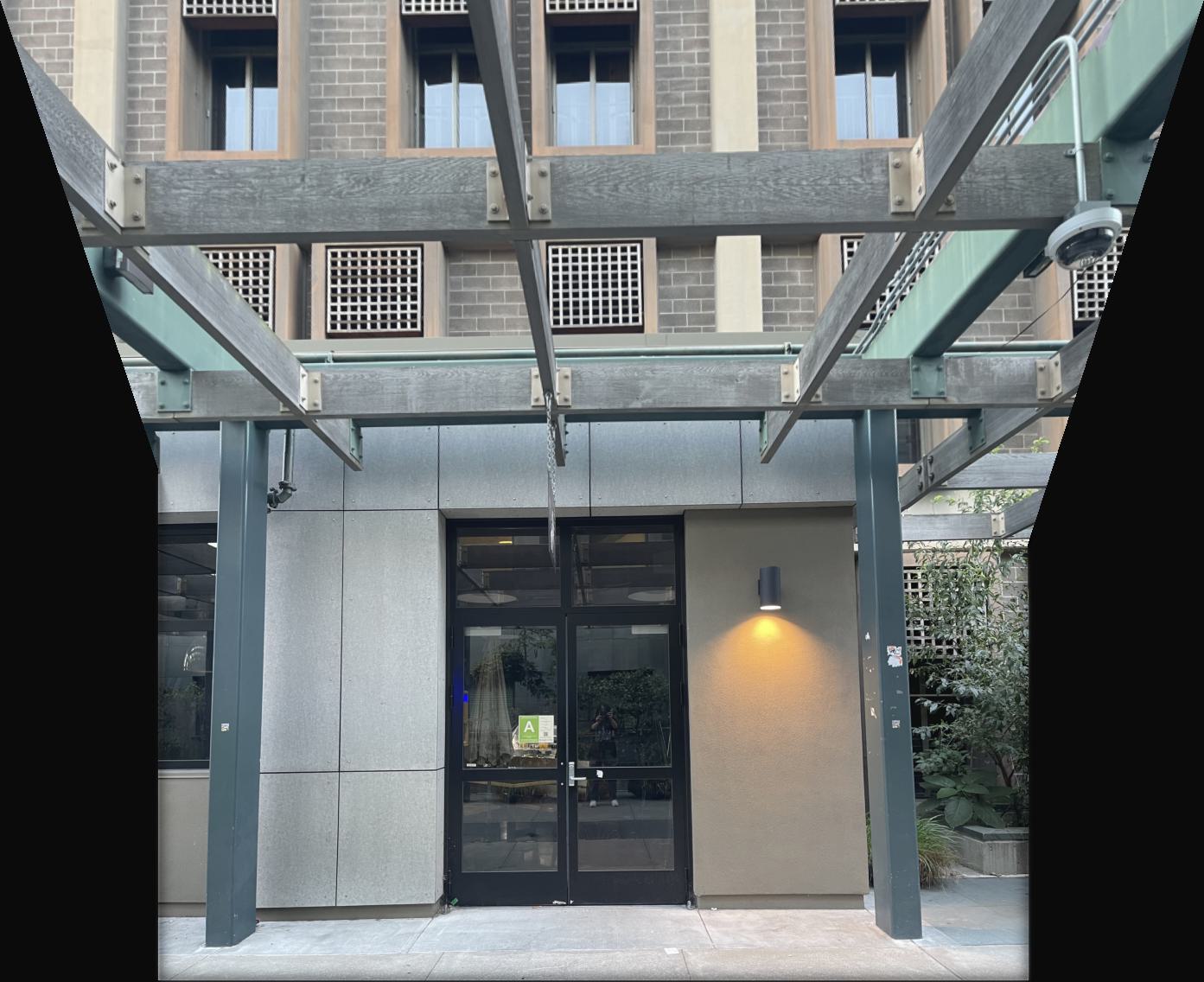
Automatically Stitched Mosaic of VA Cafe
The pillar is straight and aligned!
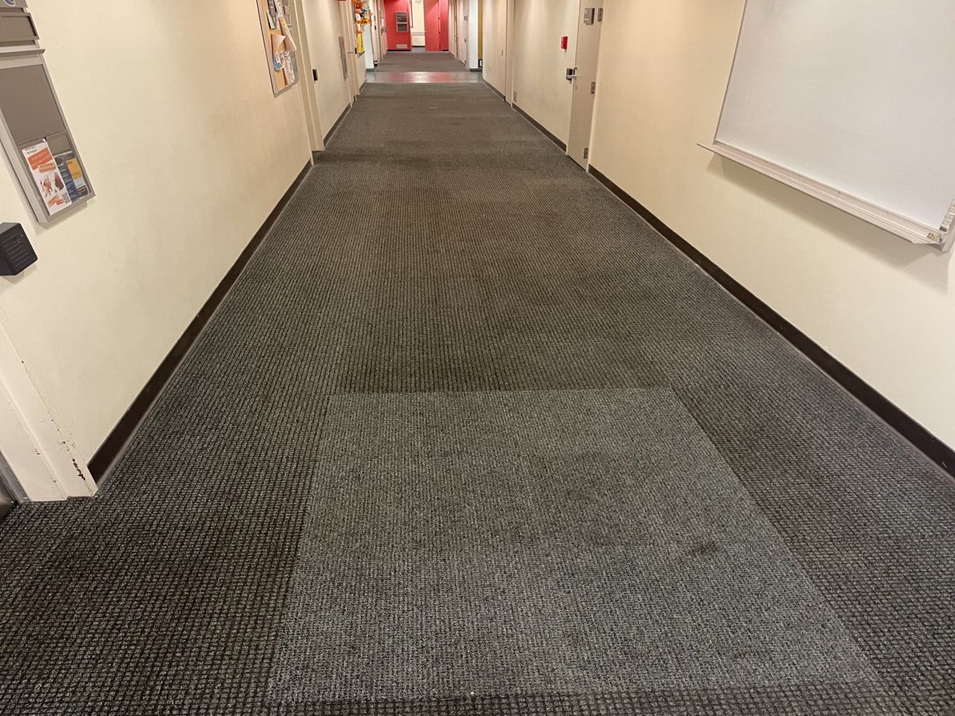
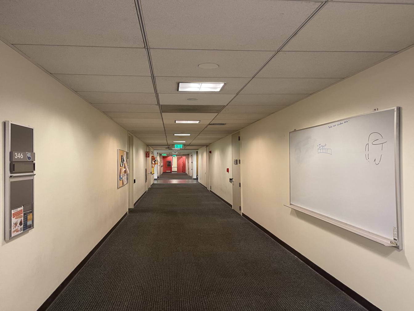
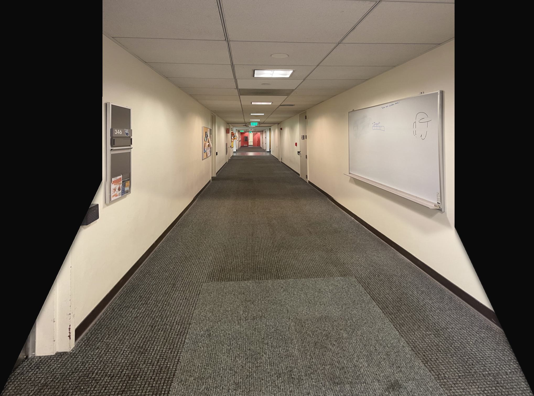
Manually Stitched Mosaic of Soda Hall Hallway
There is a slight misalignment on the left grey bulletin board thing.
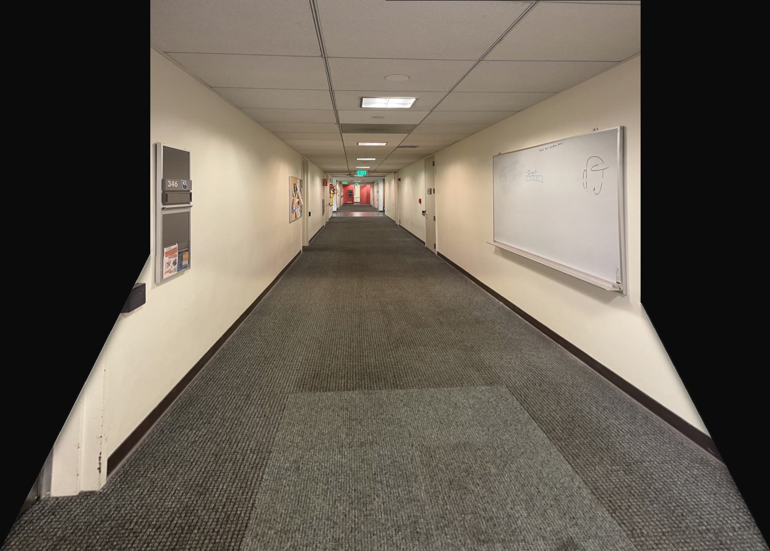
Automatically Stitched Mosaic of Soda Hall Hallway
There is still a small misalignment on the left bulletin board, but it is much less noticeable.
Reflection
Overall, this project was super interesting, as I never considered all the warping that goes into creating an image mosaic. I always assumed that all my iPhone had to do to create a panoramic photo was linearly add the images together one by one. I also thought it was very satisfying in part B to learn how to filter out more and more correspondence points through each algorithm to finally arrive at the correct set of points. For the past month, I did a lot of clicking to select correspondence points for projects 3 and 4a, and often had to start over when I realized that I clicked too hastily and the points didn't match up well, so it was really cool to learn how to automate the process. It was also interesting to look at the points that the algorithm choose, since I didn't even consider some of them, like the ones that are in the middle of a wall or chair.
